GraphSLAM Formulation

mathematical formulation for graph-based SLAM

Introduction

\(\newcommand\x{\mathbf{x}} \newcommand\xk{\mathbf{x}_k} \newcommand\xkk{\mathbf{x}_{k+1}} \newcommand\Hessian{\mathbf{H}} \newcommand\I{\mathbf{I}} \newcommand\e{\mathbf{e}}\) In the context of SLAM, we aim to estimate the optimal poses of a robot and the locations of landmarks by minimizing the error between sensor measurements and their predicted values . The optimization seeks to find the configuration of robot poses and landmark locations that minimizes the sum of the squared errors.

Formally, consider a system with:

• A set of $M$ measurements, or constraints in the graph. Each measurement $e_j \in \mathcal{E}$ is associated with:
  • An error vector $\mathbf{e}_j \in \mathbb{R}^{n_j}$, where $n_j$ is the dimensionality of the measurement error, which is dependent on the sensor type.
  • An information matrix $\Omega_j \in \mathbb{R}^{n_j \times n_j}$, representing the inverse covariance of the measurement noise.
• A set of $N$ robot poses, or vertices in the graph, $\mathcal{V} = {v_1, \dots, v_N}$. Each pose $v_i \in \mathcal{V}$ is represented by a compact state vector $\x_i \in \mathbb{R}^c$, for the 3D case, $c = 6$ and $\x = \begin{bmatrix}x,\; y,\; z,\; \phi,\; \theta,\; \psi\end{bmatrix}^\top$.
• A pose composition operator $\boxplus$ that combines pose increments $\Delta \x$ with an existing compact pose $\x$ to yield an updated (potentially non-compact) pose in $\mathbb{R}^d$ ($d \neq c$) , the work of has a detailed explanation on this operation.

Our goal is to find the set of robot poses $\x = \begin{bmatrix} \x_1, \x_2, \dots, \x_N \end{bmatrix}^{\top} \in \mathbb{R}^{cN}$ that minimizes the total squared error, the $\chi^2$ cost function: \begin{align} \chi^2(\x) = \sum_{e_j \in \mathcal{E}} \mathbf{e}_j(\x)^\top \Omega_j \mathbf{e}_j(\x). \end{align}

Back-end Formulation

This optimization problem is typically non-linear and is solved iteratively using techniques such as Gauss-Newton (GN), Levenberg-Marquardt (LM) , Powell’s dogleg (PDL) or Graduated Non-Convexity (GNC) . Let $\xk$ be the estimate of the state vector at iteration $k$. We seek an update $\Delta \xk$ such that the updated state $\xkk = \xk \boxplus \Delta \xk$ leads to a lower $\chi^2$ value.

To find this update, we linearize the error function $\e_j(\xkk)$ around the current estimate $\xk$: \begin{align} \mathbf{e}_j(\xkk) &= \mathbf{e}_j(\xk \boxplus \Delta \xk) \newline &\approx \mathbf{e}_j(\xk) + \mathbf{J}_j \Delta \xk, \end{align}

where \(\mathbf{J}_j = \left. \frac{\partial \mathbf{e}_j(\xk \boxplus \Delta \xk)}{\partial \Delta \xk} \right|_{\Delta \xk = \mathbf{0}}\) is the Jacobian matrix of the error function with respect to the state update. Using the chain rule, the Jacobian can be further decomposed as:

\[\mathbf{J}_j = \left( \left. \frac{\partial \mathbf{e}_j(\xk \boxplus \Delta \xk)}{\partial (\xk \boxplus \Delta \xk)} \right|_{\Delta \xk = \mathbf{0}} \right) \frac{\partial (\xk \boxplus \Delta \xk)}{\partial \Delta \xk}.\]

Substituting the linearized error into the $\chi^2$ cost function, we get a quadratic approximation of the error around $\xk$:

\[\begin{align} &\chi^2(\xkk) \approx \sum_{e_j \in \mathcal{E}} (\mathbf{e}_j(\xk) + \mathbf{J}_j \Delta \xk)^\top \Omega_j (\mathbf{e}_j(\xk) + \mathbf{J}_j \Delta \xk) \newline &= \sum_{e_j \in \mathcal{E}} \left[ \mathbf{e}_j(\xk)^\top \Omega_j \mathbf{e}_j(\xk) + 2 \mathbf{e}_j(\xk)^\top \Omega_j \mathbf{J}_j \Delta \xk + (\Delta \xk)^\top \mathbf{J}_j^\top \Omega_j \mathbf{J}_j \Delta \xk \right] \newline &= \chi_k^2 + 2 \mathbf{b}^\top \Delta \xk + (\Delta \xk)^\top \Hessian \Delta \xk, \end{align}\]

where the gradient vector $\mathbf{b}$ and the Hessian matrix $\Hessian$ are defined as:

\[\begin{align} \mathbf{b}^\top = \sum_{e_j \in \mathcal{E}} \mathbf{e}_j(\xk)^\top \Omega_j \mathbf{J}_j \newline \Hessian = \sum_{e_j \in \mathcal{E}} \mathbf{J}_j^\top \Omega_j \mathbf{J}_j. \end{align}\]

To find the optimal update $\Delta \xk$ that minimizes this quadratic approximation, we set the derivative with respect to $\Delta \xk$ to zero:

\begin{align} \frac{\partial \chi^2(\xkk)}{\partial \Delta \xk} = 2 \mathbf{b} + 2 \Hessian \Delta \xk = 0.
\end{align}

Solving for $\Delta \xk$, we obtain the Gauss-Newton update rule: \begin{align} \Delta \xk = -\Hessian^{-1} \mathbf{b}. \end{align}

This update is then applied to the current state estimate: $\xkk = \xk \boxplus \Delta \xk$. This iterative process continues until convergence, yielding the optimized robot poses and potentially landmark locations that best explain the sensor data.

The GN optimization technique (derived above), can converge quickly, but it can also be unstable if the initial estimate is poor. LM acts as a bridge between the GN method and the gradient descent method. It introduces a damping factor $\lambda$ to the normal equation, $(\Hessian+\lambda \I)\Delta \xk=-\mathbf{b}$. When $\lambda$ is small, it behaves such as GN, but when large, it takes smaller, more cautious steps in the direction of the gradient, making it more robust than GN, especially with poor initial estimates. Similar to LM, the PDL method also combines Gauss-Newton with gradient descent but does so by operating within a “trust region”. It calculates both the GN update and the steepest-descent update and chooses an optimal step that remains within this trusted area, providing another robust alternative to pure GN .

Key aspects of this formulation include the error function, the information matrix and the Jacobian matrix. The structure of the Hessian matrix, often sparse in large-scale SLAM problems, is crucial for efficient computation of the optimal state estimate .

A significant challenge in real-world SLAM is the presence of outliers, such as false positive loop closures, that do not fit the model. The standard least-squares formulation is highly sensitive to outliers because the error is squared, causing a single bad measurement to have a disproportionately large influence on the final solution .

To mitigate this, the error function can be wrapped in a robust cost function, or kernel, $\rho(\cdot)$. The objective function becomes: \begin{align} \chi^{2}(\x)=\sum_{\mathbf{e}_j \in \mathcal{E}}\rho(\mathbf{e}_j^\top \Omega_j \mathbf{e}_j) \end{align}

The g2o framework provides several robust kernels, with the Huber kernel being one of the most common. The Huber function is quadratic for small errors but becomes linear for large errors. This means it penalizes outliers less severely than a standard quadratic function, preventing them from corrupting the entire optimization. A key advantage of the Huber kernel is that it remains convex, which means it does not introduce new local minima into the optimization problem, ensuring more stable convergence.

This function is designed to down-weight the influence of constraints with large errors, preventing them from corrupting the optimization . The g2o framework provides several such kernels, each with different properties, as shown in the figure below:

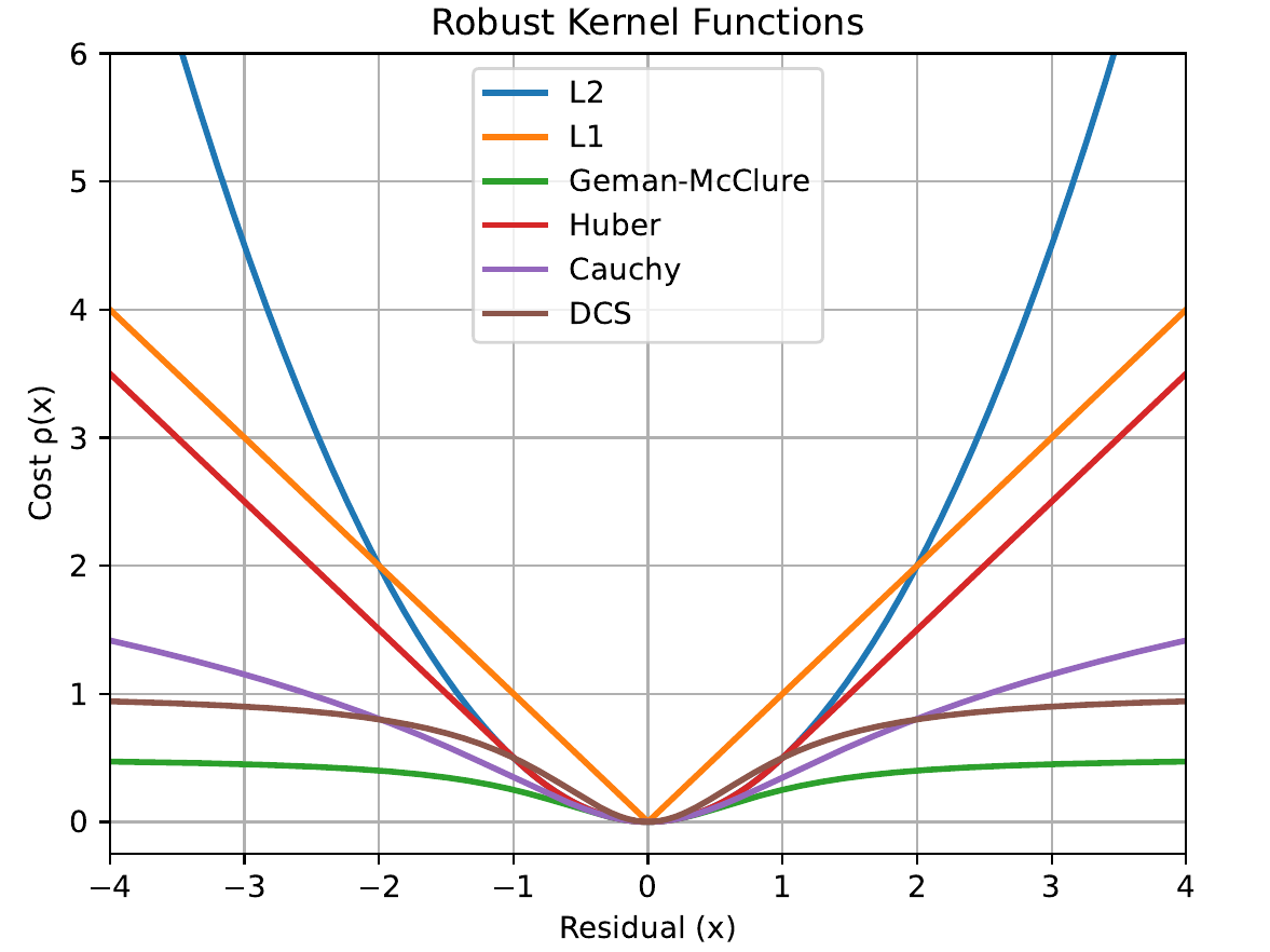
The Huber kernel is one of the most widely used robust functions. It behaves quadratically for small errors but switches to a linear function at a threshold $b$ for large errors, which prevents the error $e$ from being squared and amplified. Its formal definition is: \begin{align} \rho(e) = \begin{cases} e^{2}, & \text{if } |e| \le b \newline 2b|e| - b^{2}, & \text{otherwise} \end{cases}. \end{align}

Geman-McClure is a non-convex kernel that more aggressively suppresses the influence of large errors. As the error $\e$ increases, the cost function flattens out and approaches a constant value $b$, effectively ignoring measurements that are considered strong outliers. Its formula is:
\begin{align}
\rho(e)=\frac{\frac{e^{2}}{2}}{(b+e^{2})}. \end{align}

Dynamic Covariance Scaling (DCS) takes a different approach by introducing an additional scaling factor $s$ that directly modifies the information matrix for each loop closure constraint, as shown in the equation below. The scaling factor is close to 1 for inliers but drops towards zero for outliers, effectively down-rating their influence on the optimization . The scaling factor is defined as:
\(\begin{align} \sum \mathbf{e}_{\text{lc}}(\x)^\top (s^2 \Omega_{\text{lc}}) \; \mathbf{e}_{\text{lc}}(\x), \newline s = \min\Bigg(1, \frac{2\Phi}{\Phi+\chi_{\text{lc}}^2}\Bigg) \end{align}\)

where \(\mathbf{e}_{\text{lc}}\) is the loop closure constraint, \(\Omega_{\text{lc}}\) is the loop closure information matrix, $\Phi$ is a parameter defining the influence of the down-rate and $\chi_{\text{lc}}^2$ is the original term for the loop closure constraint.

Other robust functions such as the Cauchy, Tukey, and Welsh kernels also exist, each offering a different non-convex strategy for down-weighting outliers. The choice of kernel is ultimately a trade-off between the desired level of robustness to extreme outliers and the stability of the optimization process. While non-convex kernels can offer better performance in the presence of severe outliers, convex options such as Huber are often preferred for their reliability and predictable behavior. Experiments show that robust kernels dramatically improve accuracy when initial estimates are poor or when data contains incorrect constraints .

---

Front-end Formulation

Coming soon…